Note: Superseded by Get started with Charmed Kubeflow | Documentation | Charmed Kubeflow . Please see that doc instead.
This documentation was written for Charmed Kubeflow based on Kubeflow 1.4 and Katib 0.12.
Contents:
- Using Kubeflow - Basic
- Get to know the Dashboard
- Creating a Kubeflow Notebook
- Visualize your notebook experiments with Tensorboard
- Adding Kubeflow Pipelines
- Using Kubeflow Kale
- Running experiments with Katib
Using Kubeflow - Basic
Congratulations on installing Kubeflow! This page will run through setting up a typical workflow to familiarise you with how Kubeflow works.
These instructions assume that :
-
You have already installed Kubeflow on your cluster (full or lite version).
-
You have logged in to the Kubeflow dashboard.
-
You have access to the internet for downloading the example code (notebooks, pipelines) required.
-
You can run Python 3 code in a local terminal (required for building the pipeline).
This documentation will go through a typical, basic workflow so you can familiarise yourself with Kubeflow. Here you will find out how to:
-
Create a new Jupyter notebook
-
Add a Tensorflow example image
-
Create a pipeline
-
Start a run and examine the result
Get to know the Dashboard
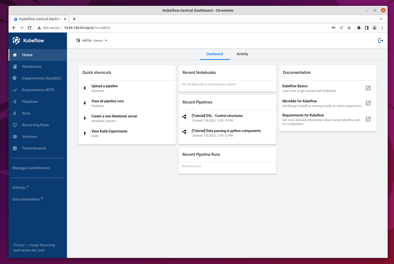
The Kubeflow Dashboard combines some quick links to the UI for various components of your Kubeflow deploy (Notebooks, Pipelines, Katib) as well as shortcuts to recent actions and some handy links to the upstream Kubeflow documentation.
Creating a Kubeflow Notebook
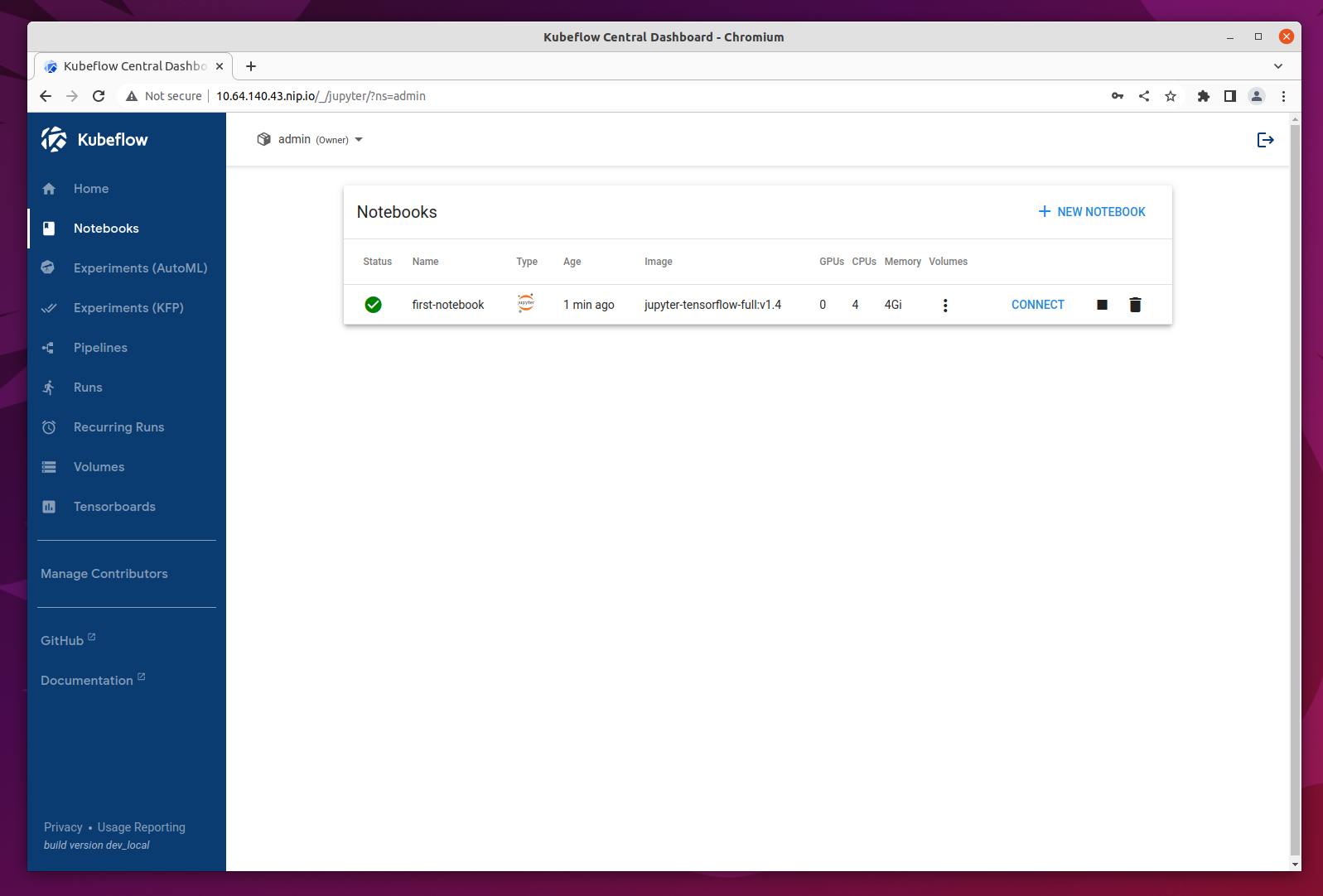
This Dashboard will give you an overview of the Notebook Servers currently available on your Kubeflow installation. In a freshly installed Kubeflow there will be no Notebook Server.
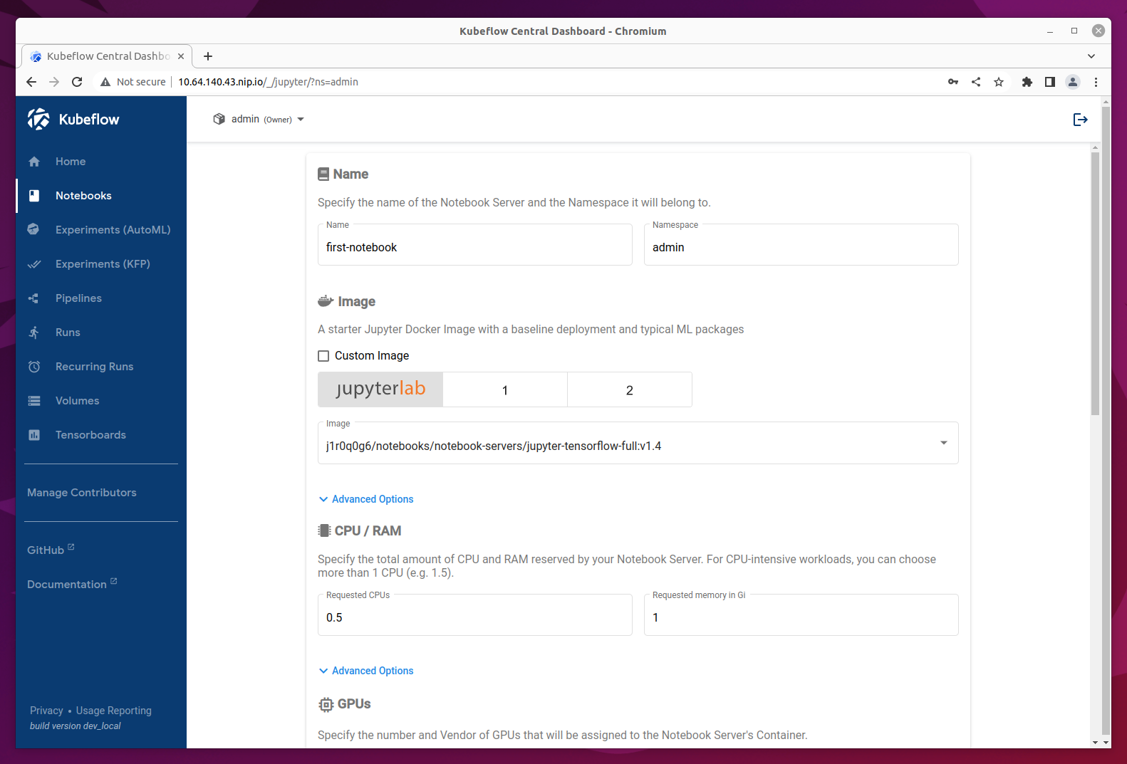
You can create a new Notebook Server by clicking on Notebooks in the left-side navigation and then clicking on the New notebook button.
In the New Notebook section you will be able to specify several options for the notebook you are creating. In the image section choose an image of jupyter-tensorflow-full, it is required for our example notebook. Consider bumping the default CPU and memory values to speed up your notebook.
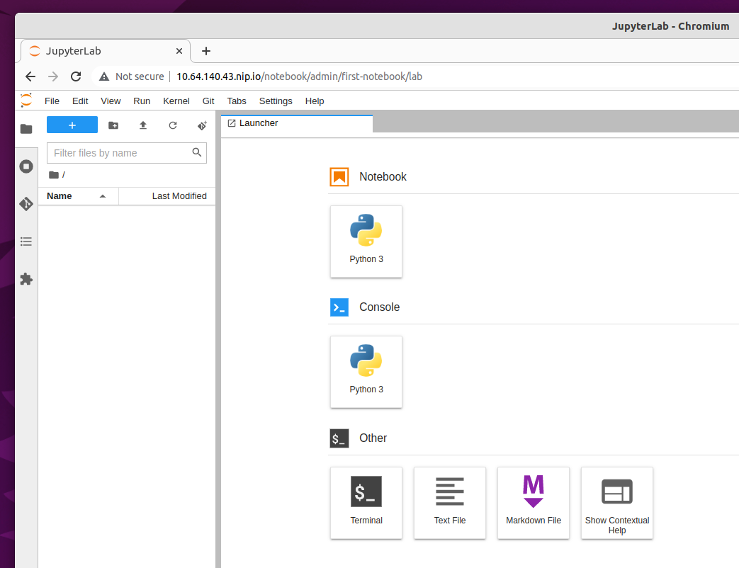
Once the Notebook Server is created you will be able to connect to it and access your Jupyter Notebook environment which will be opened in a new tab.
For testing the server we will upload the Tensorflow 2 quickstart for experts example.
Click on the link above and click on the Download Notebook button just below the heading. This will download the file advanced.ipynb into your usual Download location. This file will be used to create the example notebook.
On the Notebook Server page, click on the Upload button and select the advanced.ipnyb file.
Once uploaded, click on the notebook name to open a new tab with the notebook content.
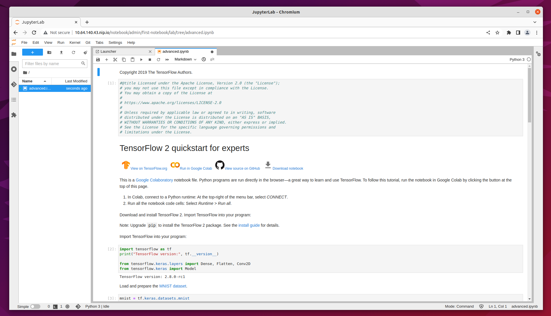
You can read through the content for a better understanding of what this notebook does. Click on the Run button to execute each stage of the document, or click on the double-chevron (>>) to execute the entire document.
Visualize your notebook experiments with Tensorboard
Tensorboard provides a way to visualise your ML experiments. It can track metrics such as loss and accuracy, view histograms of biases, model graphs and much more. You can learn more about the project on the upstream website.For a quick example, you can reuse the notebook server created in previous step. Connect to it and upload a new notebook for Tensorboard Download the notebook here.
Note the log_dir path - this location will be needed for Tensorboad creation.
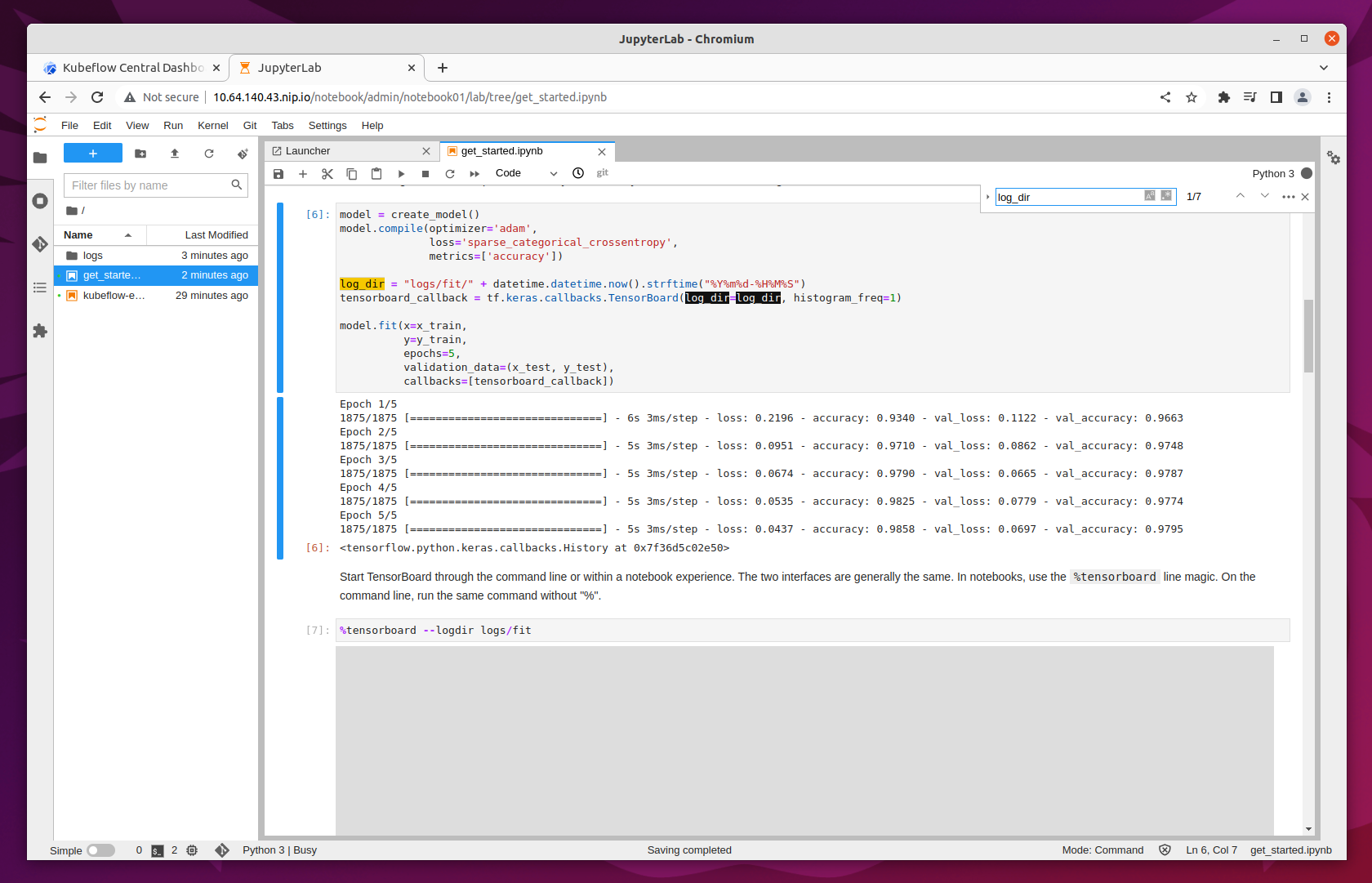
Run the notebook and navigate to Tensorboards.
Click on New Tensorboard. Name it and select the PVC checkbox. Select your notebook’s workspace volume from the dropdown list and fill in the Mount Path field with the log_dir you have noted in the previous step. In our example it’s logs/fit.
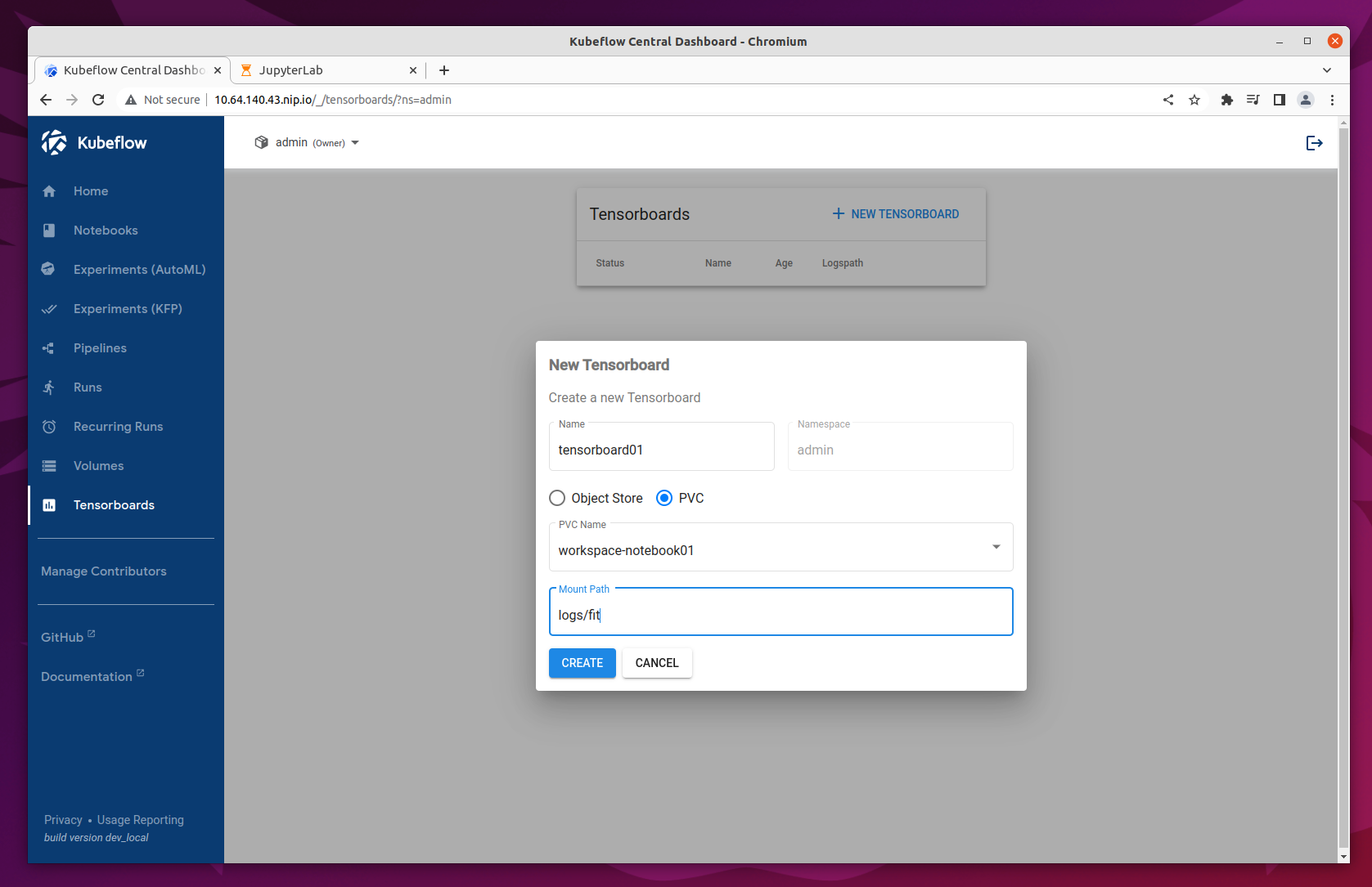
That’s it! Click on Create and your Tensorboard should be up and running within minutes.
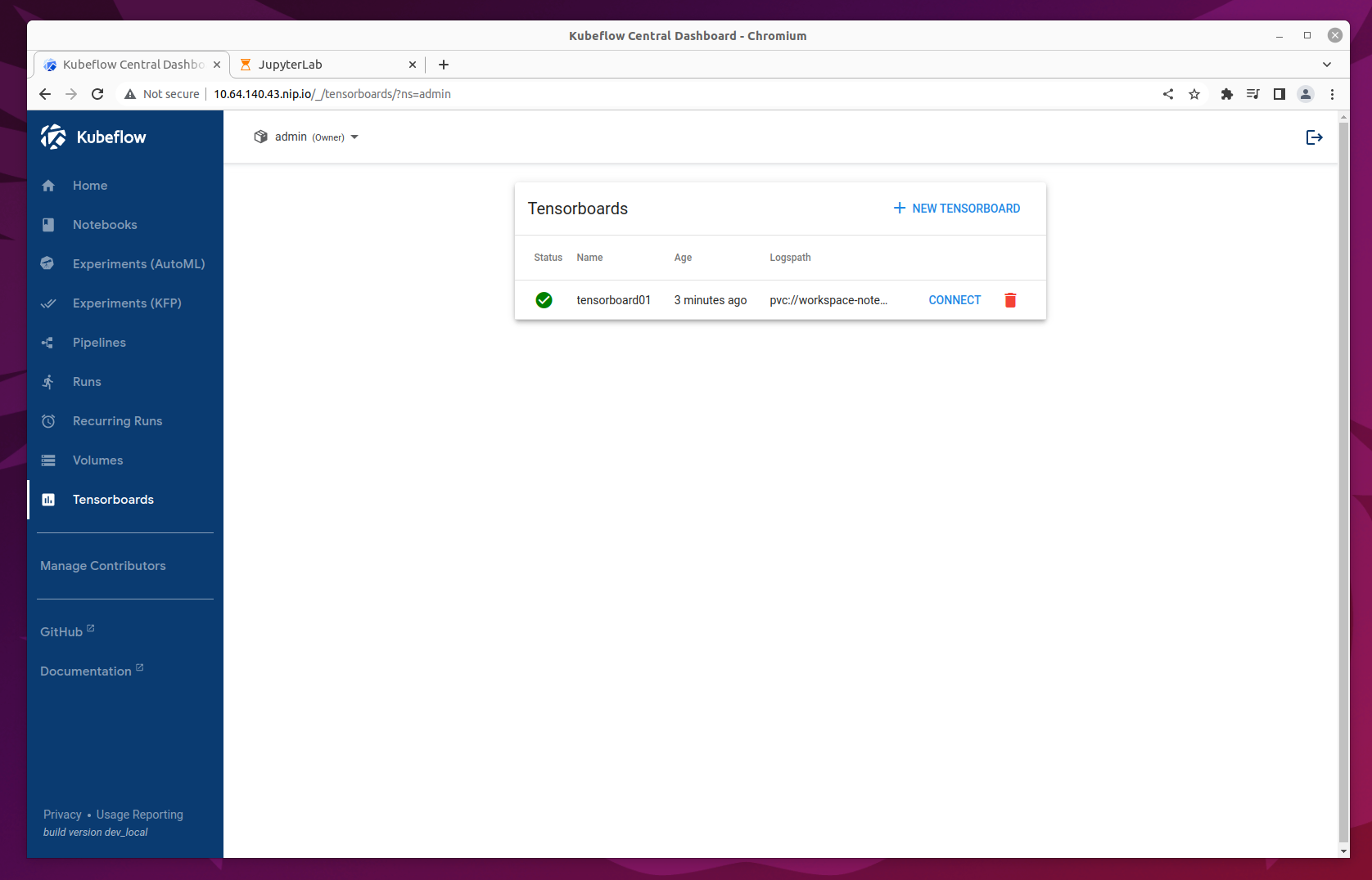
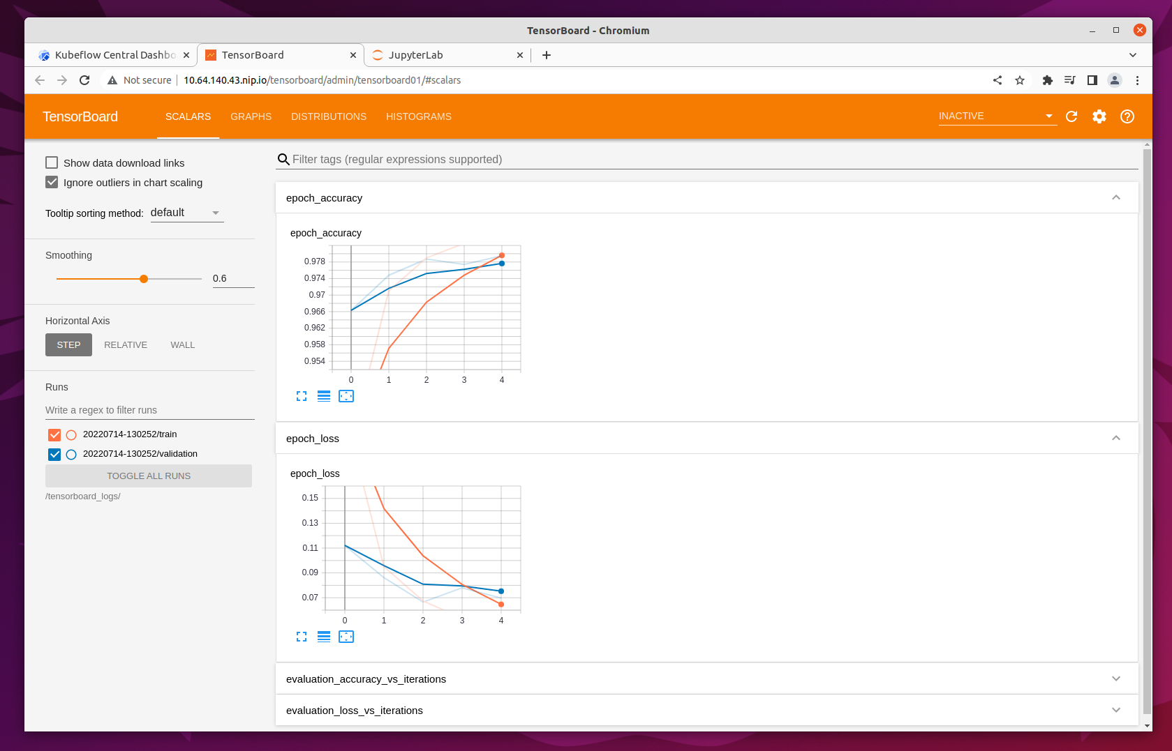
You can then connect to it and see various metrics and graphs.
Adding Kubeflow Pipelines
The official Kubeflow Documentation explains the recommended workflow for creating a pipeline. This documentation is well worth reading thoroughly to understand how pipelines are constructed. For this example run-through though, we can take a shortcut and use one of the Kubeflow testing pipelines.If you wish to skip the step of building this pipeline yourself, you can instead download the compiled YAML file.
To install the pipeline compiler tools, you will need to first have Python 3 available, and whichever pip install tool is relevant for your OS. On Ubuntu 20.04 and similar systems:
sudo apt update

sudo apt install python3-pip
Next, use pip to install the Kubeflow Pipeline package
pip3 install kfp
(depending on your operating system, you may need to use pip instead of pip3 here, but make sure the package is installed for Python3)
Next fetch the Kubeflow repository:
git clone https://github.com/juju-solutions/bundle-kubeflow.git
The example pipelines are Python files, but to be used through the dashboard, they need to be compiled into a YAML. The dsl-compile command can be used for this usually, but for code which is part of a larger package, this is not always straightforward. A reliable way to compile such files is to execute them as a python module in interactive mode, then use the kfp tools within Python to compile the file.
First, change to the right directory:
cd bundle-kubeflow/tests
Then execute the pipelines/mnist.py file as a module:
python3 -i -m pipelines.mnist
With the terminal now in interactive mode, we can import the kfp module:
import kfp
… and execute the function to compile the YAML file:
kfp.compiler.Compiler().compile(mnist_pipeline, 'mnist.yaml')
In this case, mnist_pipeline is the name of the main pipeline function in the code, and mnist.yaml is the file we want to generate.
Once you have the compiled YAML file (or downloaded it from the link above) go to the Kubeflow Pipelines Dashboard and click on the Upload Pipeline button.
In the upload section choose the “Upload a file” section and choose the mnist.yaml file. Then click “Create” to create the pipeline.

Once the pipeline is created we will be redirected to its Dashboard. Create an experiment first:

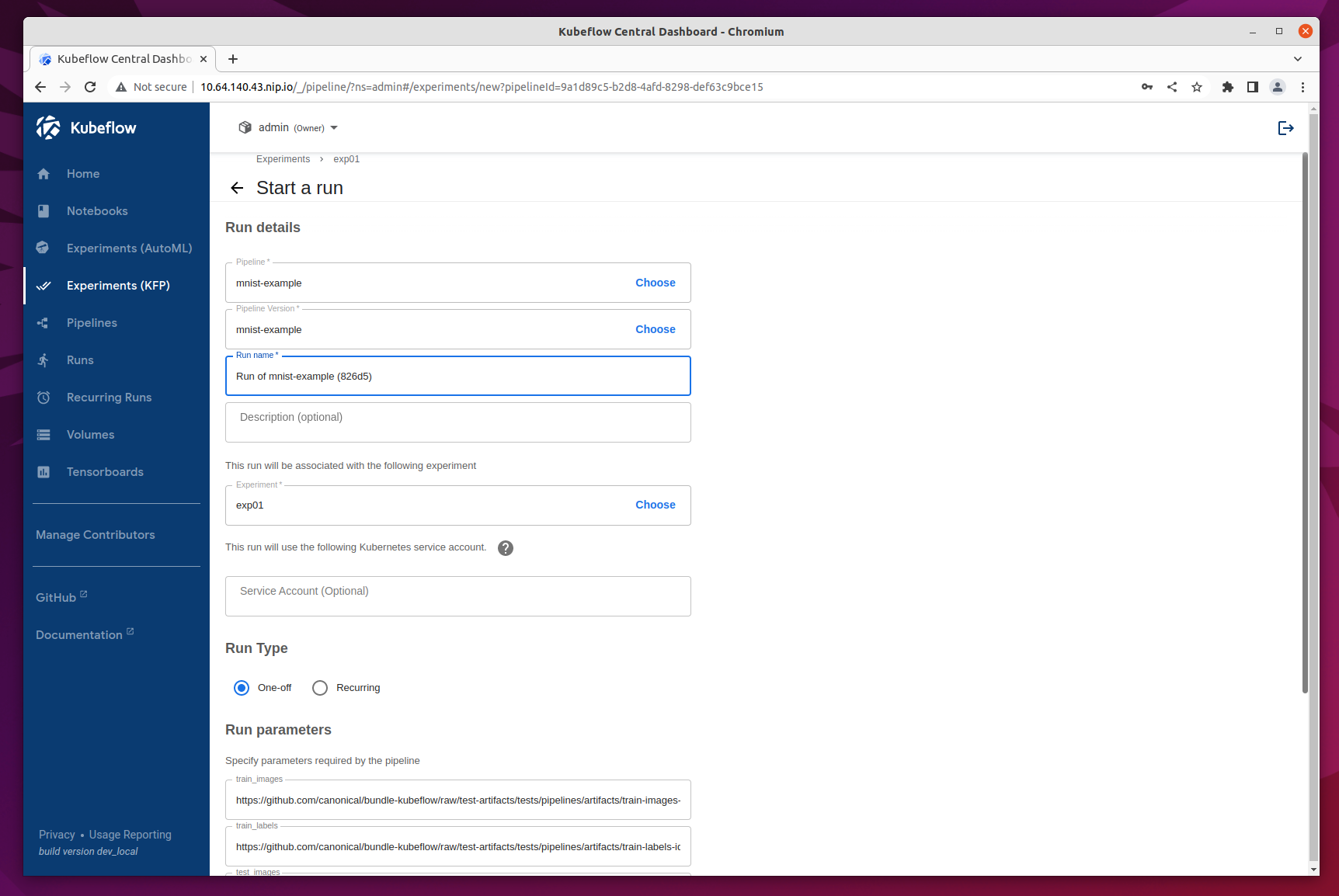
Once the experiment is added, you will be redirected to Start a Run.
For this test select ‘One-off’ run and leave all the default parameters and options. Then click Start to create your first Pipeline run!
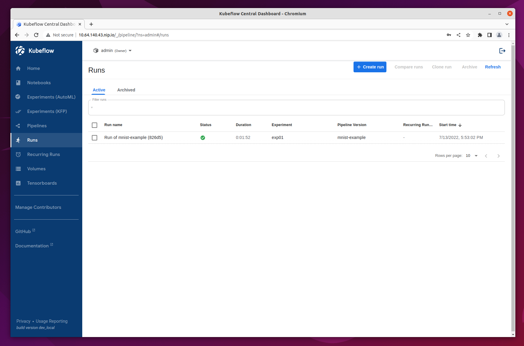
Once the run is started, the browser will redirect to Runs, detailing all the stages of the pipeline run. After a few minutes there should be a checkpoint showing that it has been executed successfully.
Using Kubeflow Kale
Kale is a project that makes it easy to create a pipeline from a notebook server. The recommended way of using Kale is to input a custom image when creating a notebook server that includes kale built-in. Here is an example custom image and how to use it: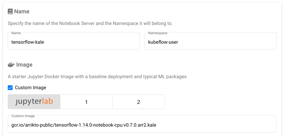
The upstream default jupyterlab Dockerfile is available as:
rocks.canonical.com:5000/kubeflow/notebook-kale:bda9d296
After the notebook server starts up, you can open the Kale dashboard from the side menu:
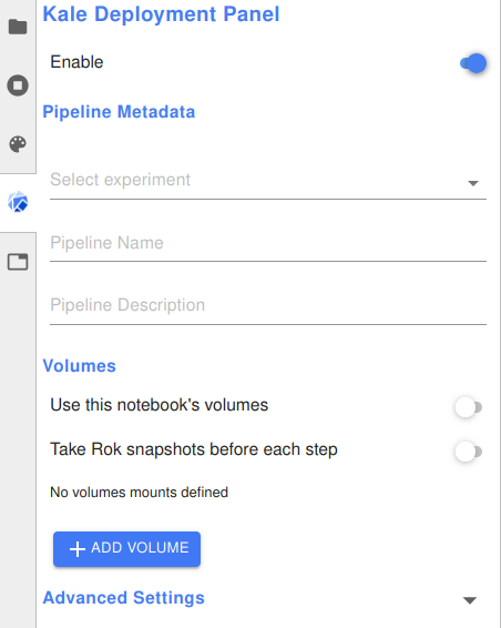
Note that Kale is not currently up-to-date with the latest version of jupyterlab, so you cannot install it into a notebook server you have already created, you need to use a pre-built docker image that includes Kale.
Running experiments with Katib
Using Katib:
Katib is not deployed by default with kubeflow-lite. To enable it, follow the customisation tutorial.
If you are unfamiliar with Katib and hyperparameter tuning, plenty of information is available on the upstream Kubeflow documentation. In summary, Katib automates the tuning of machine learning hyperparameters - those which control the way and rate at which the AI learns; as well as offering neural architecture search features to help you find the optimal architecture for your model. By running experiments, Katib can be used to get the most effective configuration for the current task.
Each experiment represents a single tuning operation and consists of an objective (what is to be optimised), a search space(the constraints used for the optimisation) and an algorithm(how to find the optimal values).
You can run Katib Experiments from the UI and from CLI.
For CLI execute the following commands:
curl https://raw.githubusercontent.com/kubeflow/katib/master/examples/v1beta1/hp-tuning/grid.yaml > grid-example.yaml

yq -i '.spec.trialTemplate.trialSpec.spec.template.metadata.annotations."sidecar.istio.io/inject" = "false"' grid-example.yaml

kubectl apply -f grid-example.yaml
the yq command is used to disable istio sidecar injection in the .yaml, due to its incompatibility with Katib experiments. Find more details in upstream docs.
If you are using a different namespace than kubeflow make sure to change that in grid-example.yaml before applying the manifest.
These commands will download an example which will create a katib experiment. We can inspect experiment progress using kubectl by running the following command:
kubectl -n kubeflow get experiment grid-example -o yaml
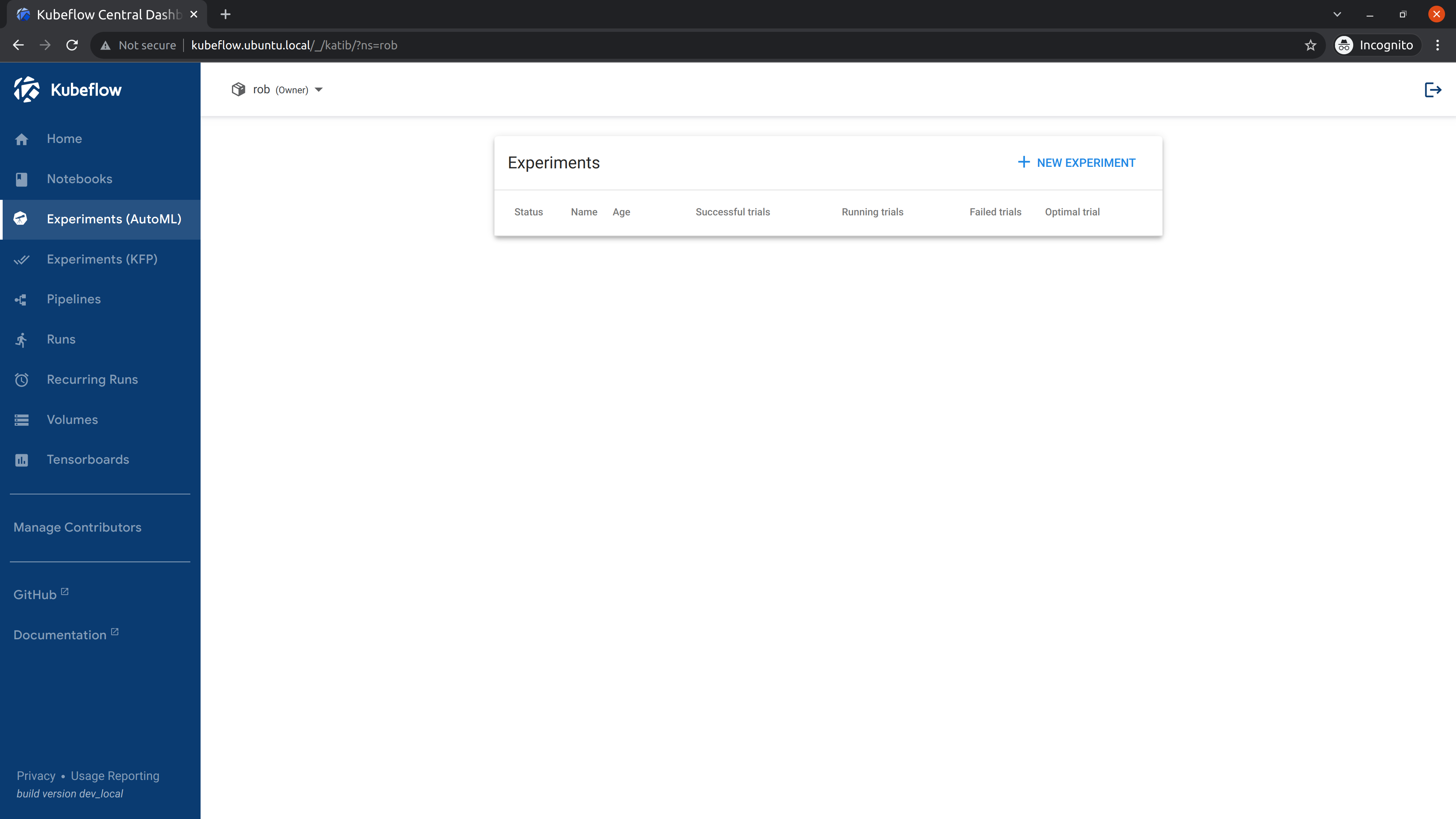
We can also use the UI to run the same example. Go to Experiments (AutoML), and select “New Experiment”.
Save the contents of this YAML file as grid-example.yaml. Open it and edit it, adding sidecar.istio.io/inject="false" under .spec.trialTemplate.trialSpec.spec.template.metadata.annotations as shown here:
---
apiVersion: kubeflow.org/v1beta1
kind: Experiment
metadata:
  name: grid
spec:
  objective:
    type: maximize
    goal: 0.99
    objectiveMetricName: Validation-accuracy
    additionalMetricNames:
      - Train-accuracy
  algorithm:
    algorithmName: grid
  parallelTrialCount: 1
  maxTrialCount: 1
  maxFailedTrialCount: 1
  parameters:
    - name: lr
      parameterType: double
      feasibleSpace:
        min: "0.001"
        max: "0.01"
        step: "0.001"
    - name: num-layers
      parameterType: int
      feasibleSpace:
        min: "2"
        max: "5"
    - name: optimizer
      parameterType: categorical
      feasibleSpace:
        list:
          - sgd
          - adam
          - ftrl
  trialTemplate:
    primaryContainerName: training-container
    trialParameters:
      - name: learningRate
        description: Learning rate for the training model
        reference: lr
      - name: numberLayers
        description: Number of training model layers
        reference: num-layers
      - name: optimizer
        description: Training model optimizer (sdg, adam or ftrl)
        reference: optimizer
    trialSpec:
      apiVersion: batch/v1
      kind: Job
      spec:
        template:
          metadata:
            annotations:
              sidecar.istio.io/inject: "false"
          spec:
            containers:
              - name: training-container
                image: docker.io/kubeflowkatib/mxnet-mnist:latest
                command:
                  - "python3"
                  - "/opt/mxnet-mnist/mnist.py"
                  - "--batch-size=64"
                  - "--lr=${trialParameters.learningRate}"
                  - "--num-layers=${trialParameters.numberLayers}"
                  - "--optimizer=${trialParameters.optimizer}"
            restartPolicy: Never
Refer to the previous section using CLI for clarification on adding this field.
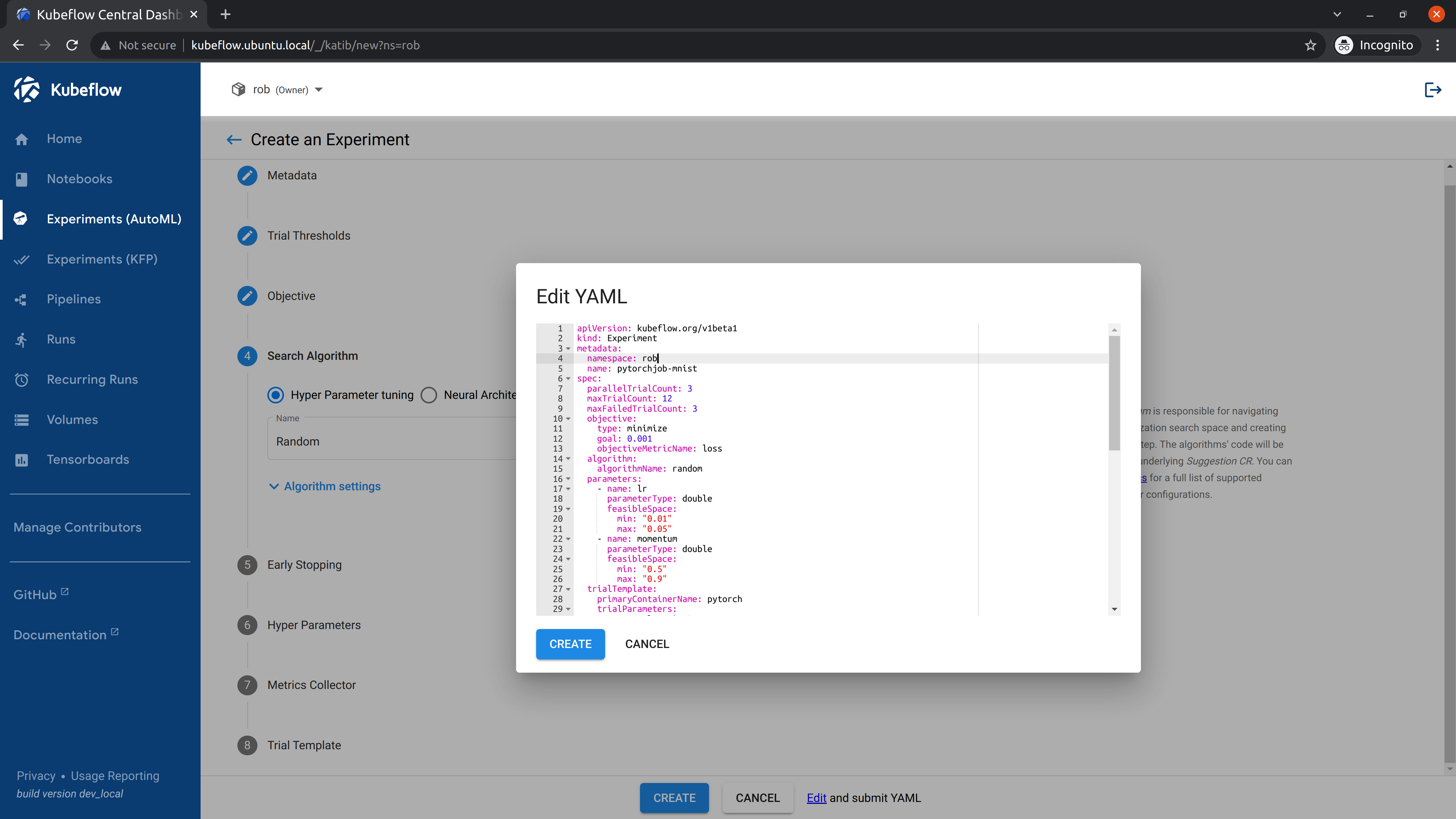
Click the link labelled “Edit and submit YAML”, and paste the contents of the yaml file.
Remember to change the namespace field in the metadata section to the namespace where you want to deploy your experiment.
Afterwards we will click Create.
Once the experiment has been submitted, go to the Katib Dashboard and select the experiment.
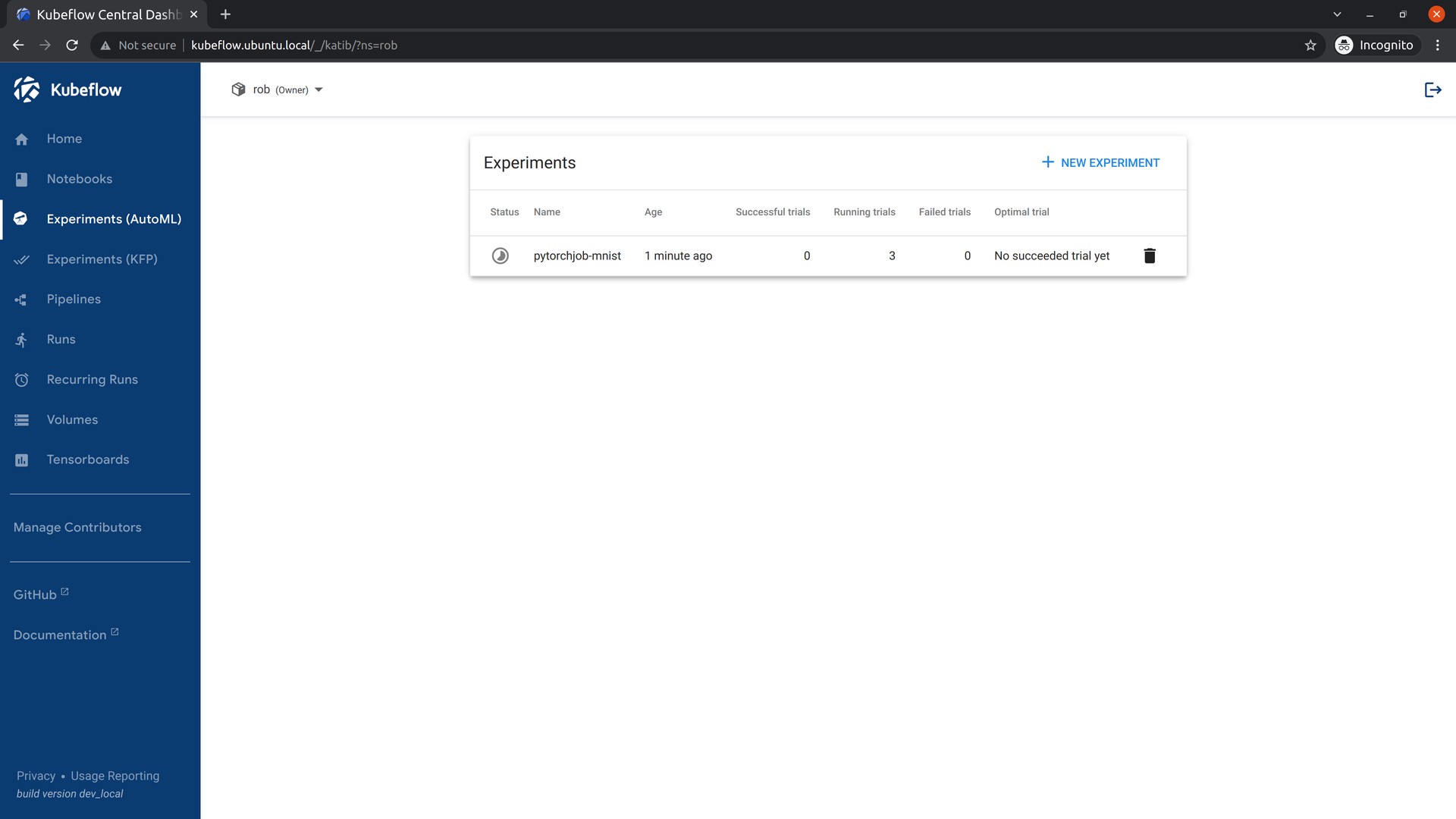
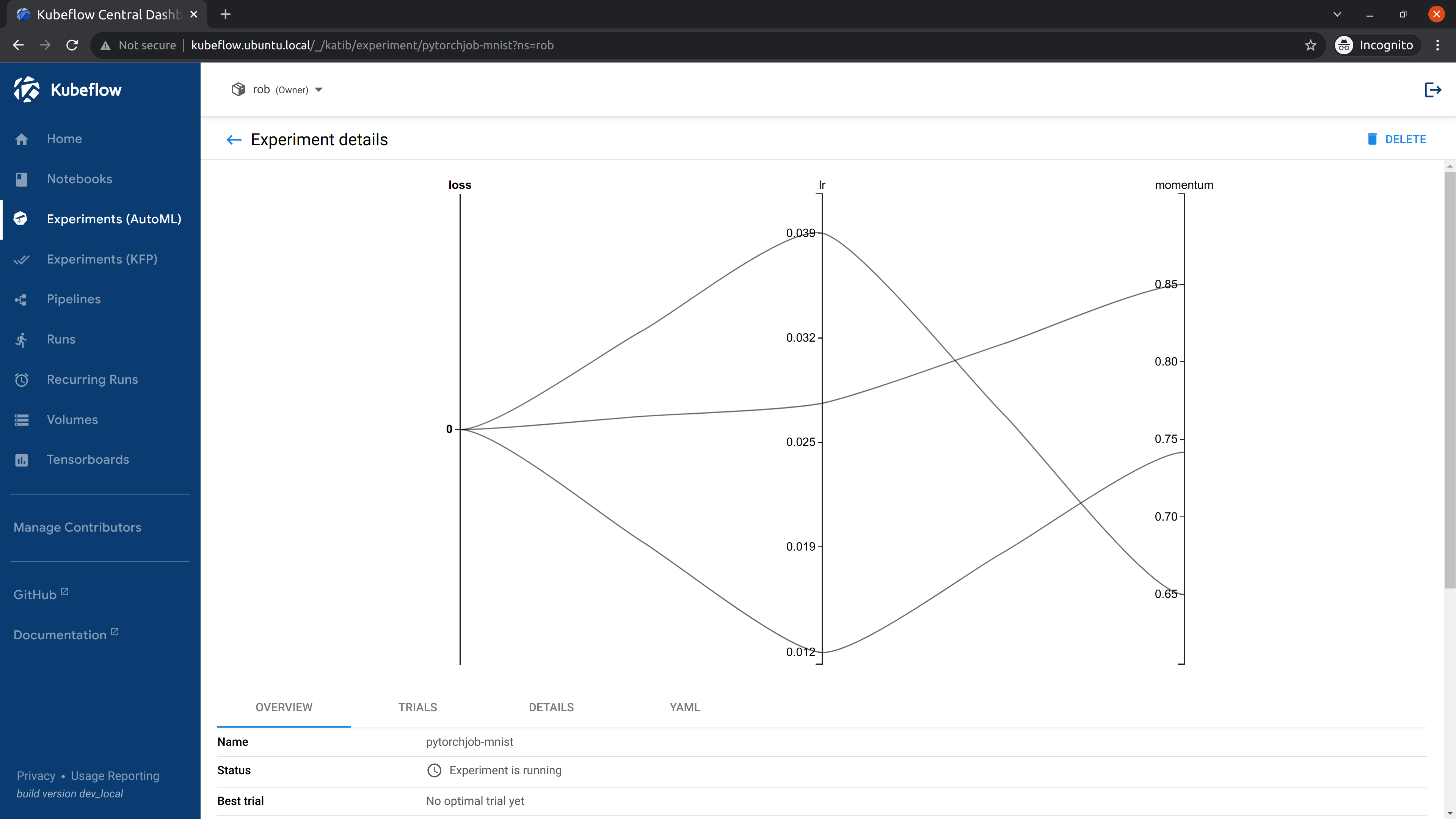
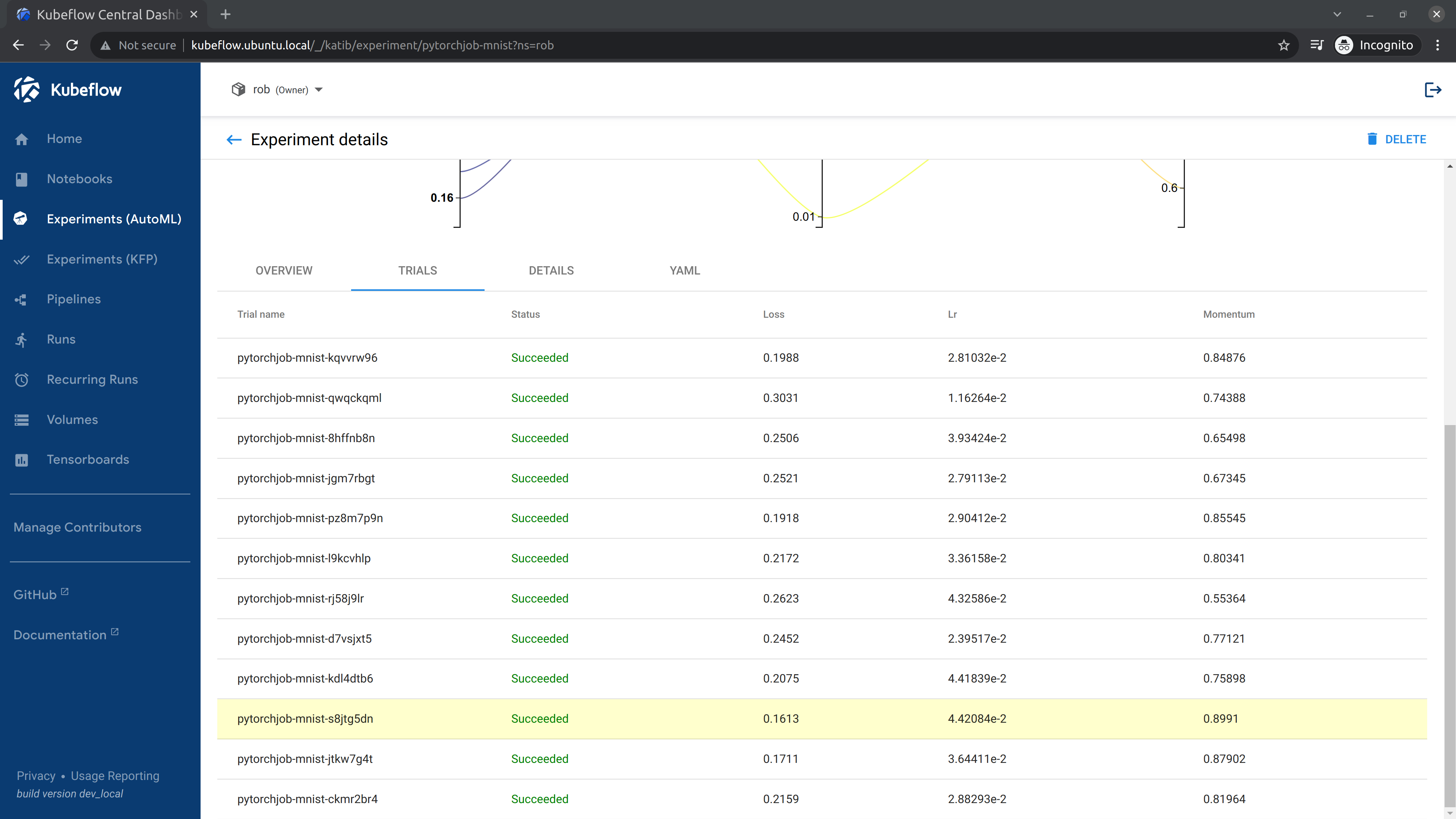
In the Experiment Details view, you can see how your experiment is progressing.
When the experiment completes, you will be able to see the recommended hyperparameters.
Next steps
This has been a very brief run through of the major components of Kubeflow. To discover more about Kubeflow and its components, we recommend the following resources:
- The upstream Kubeflow Documentation.